Activities · Teaching Methods

Paper Companion Activities for Pivot Interactives

You know how I feel about online work! (Looking for Physics Classroom Companion Worksheets? Find them Here!)

When I took high school physics almost everything was online. From physics classroom assignments, to the dreaded WebAssign, it was online. And because it was online, I like others, gamed the system (pre chat GPT). You know a certain number is going to show up somewhere in the answers? Enter it in all the blanks for the first submission so you can focus on the actual calculations. On the flip side was the part where you tried the problem so many times by the time you got it right you had no idea what actually worked. For the better part of my career I’ve been vehemently against all forms of online homework. There’s something about that screen that just puts a stop to the idea of using scratch paper for novice learners and we can’t have that!

(For what it’s worth, when AP went all digital I did NOT feel the urge to go digital in my classroom. I continued to do everything on paper. When APs came around I found my goal was acheived: I proctored the macro exam and did a count. 80% of physics students were using their scratch paper during the exam, while only 30% of non-physics students used their paper.)

The first exception I made to online learning was Pivot Interactives. I was using Peter’s work back when they were “Direct Measurement Videos” which meant I had paper copies originally, anyway. As Pivot upped their game (including deep randomization and autograding) I started using some of these assignments since it sure made my life easier!

However, what I’m finding with my students this year is that like my Webassign days, students are doing the minimum to get all the green checks. This looks like not reading the prompts that explain what they’re about to do next and why, not actually collecting the data for the graph and totally missing the connections between the sample measurements and the data collection.

So, I’ve started to reimplement some paper versions.

The Activities: A Journey of Trial and Error

Earlier this year I assigned the helmet collisions activity. I added a prompt at the end that requested students to do the following:

  • What was the purpose of the activity?
  • Describe the procedure for conducting the investigation
  • Describe the calculations you made and why we made each calculation. You should include details regarding your values!
  • Describe what we learned from this activity about helmets as it relates to the impulse-change in momentum relationship.

This was ok, but I, arguably did this a bit hastily. I realized I wanted these documents handwritten and maybe a bit more depth/scaffholding.

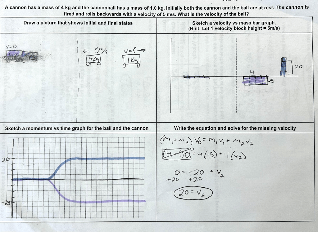
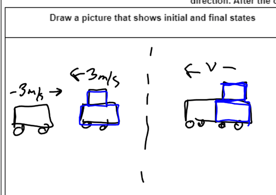
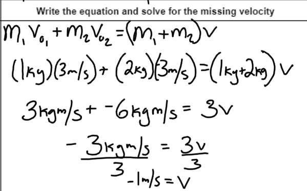
A few weeks later I assigned the Explosions (Not Really) activity.

I knew that students would totally ditch all of the methods we had been using, so I decided to give them a paper to complete before the activity that related to the activity. This required them to complete the calculations with similar, but easy numbers and then have me check their work prior to the activity. This got a good chunk of kids on board, but some still struggled with the transference.

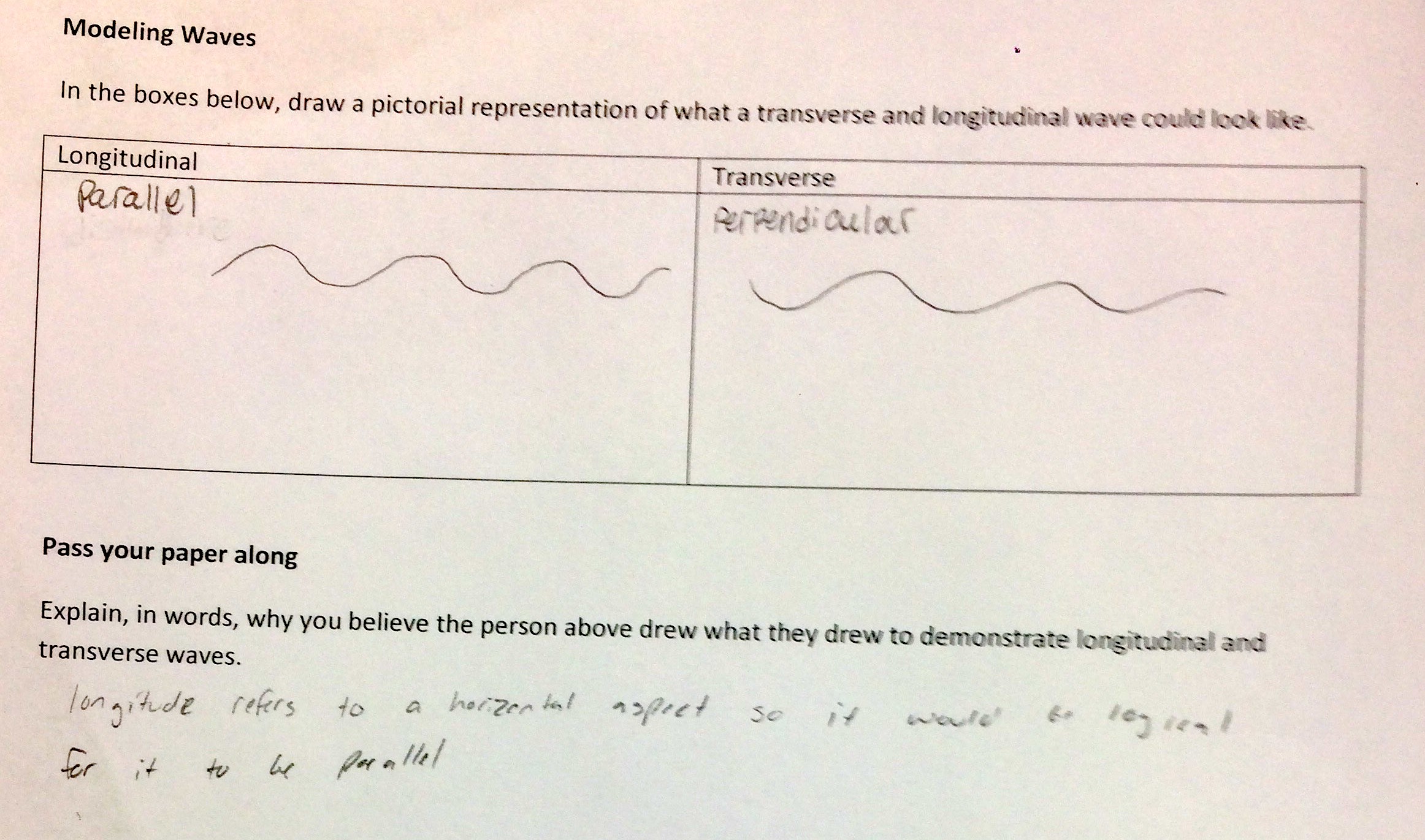
Still not completely satisfied, this past week I assigned the “Intro to Transverse Waves” activity. In this activity students are going to linearize a graph. This is a skill we don’t really cover in my regular level physics, but I like doing it at this point in the year because it’s such a powerful tool. As I anticipated, many students were ignoring the text about linearization completely. I chose a different approach to the paper copy.

I gave students this document which contains the following prompts:

First, I asked them to describe to me some of the new vocab as well as how we obtained our measurements

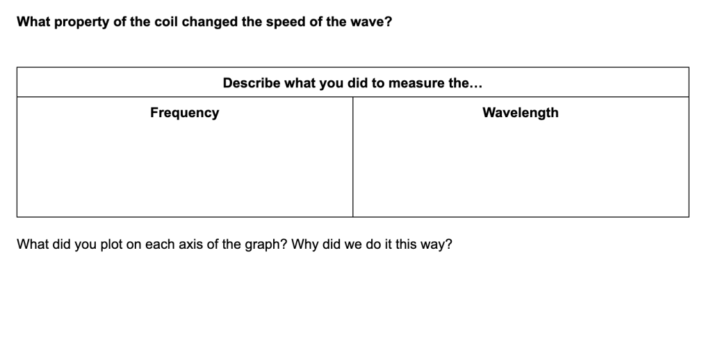
Next, I use a modified template from the Patterns Curriculum when students write conclusions in labs where we have graphs. It looks like this:

After investigating the behavior _______________, I conclude that there is a ______________________relationship between the [independent variable name]  and the [dependent variable name] As the [independent variable] kept increasing, the [dependent variable]_____________________________. This system of a ___________________ can be mathematically modeled as:

[write the final equation]

where the constant  [slope value]  is the [description of slope for this experiment]

I require students to write the ENTIRE paragraph from start to finish. This is not a fill in the blank activity.

This is currently my favorite interaction of the paper follow up and I’ll probably build more of these moving forward. I’m really in love with the patterns physics conclusions because it really requires students to put everything together.

Grading

I’ve noticed there’s a VERY strong correlation on these summaries between students who took the activity seriously and learned from it, vs students who did not. Because of this, the only thing I really need to grade with care is the conclusion paragraph itself. If students did the lab correctly, this paragraph looks great. If not, they usually don’t do well on this.

Do you do anything like this? What does it look like? How do you support genuine learning using online platforms?

Activities · Teaching Methods

I revised the cannon launch!

In my last post I talked about how I finally reenvisioned collisions and explosion problem solving for my on-track physics. It went so well I’m definitely going to integrate more of it into AP.

The goal of the reenvisioning was to set students up for a meaningful tennis ball cannon launch lab at the end of the lesson sequence.

If you’re unfamiliar, you create a tennis ball cannon, launch it, and have students calculate some quantity based on momentum conservation. To be honest, I haven’t run this lab since my first few years teaching for a few reasons. One was that my cannon got stolen at my first job. Then I decided that whole class labs are less effective than small group work and I hate when it looks like everyone is copying answers. The activity just wasn’t meaningful enough.

But after talking to several friends, everyone was excited about the idea of a cannon launch, so I spent my weekend rebuilding a cannon.

To open the lesson I set up and demonstrated an “explosion” with our car-track system. I ensured that one car had more mass than the other and we had some conversations about what to expect. We also talked about what the equation would look like based on our previous experiences with elastic and inelastic collisions. Students were able to correctly determine that it’s basically the opposite of an inelastic collision.

Next, I gave them the scenario where the cannon had a mass of 4.0 kg, the ball had a mass of 1.0 kg and the cannon’s launch velocity was 5 m/s. These numbers were strategically chosen. I wanted to keep whole numbers and also have a cannon-ball ratio that was similar to the actual cannon-tennis ball.

Students then completed the four representations as we’d previously done earlier in the week. Below is a student work sample.

The great thing about this was that students were able to accurately represent and predict the outcomes of the cannon-ball system before we got into the muck. This got students thinking individually and talking in small groups. We also discussed why the results made sense.

To launch the cannon I let it go through a photogate to snag the post explosion velocity and then students completed the calculations.

For the post-lab analysis I threw in a few thinkers. They included:

  • Find the average force on the ball
  • How would a longer cannon change the ball’s launch speed? Explain in terms of impulse-momentum
  • If we used the same cannon but filled the tennis ball with rice, what would happen to the speeds of the ball and cannon post explosion?

You can see a sample student response below:

These questions led to some really great conversations that brought us back to equal forces, equal momentum changes and where time falls into the mix.

Concept Modeling · In My Class Today · Teaching Methods

Multiple Representations for Momentum Conservation

I did it. I finally revised how I teach momentum conservation to my on-track physics students and I’m never looking back!

It can be really hard to shift something that “works” especially if you don’t have a team. For my on-track physics students collision/explosion problems were always an “easy win” for students. We would define that “momentum is conserved” and then talk about how to solve the problems. I would lecture and show them the “table method” and then the “brute force method” and allow them to choose how they wanted to solve.

This was satisfying for students. It felt easy and students gained confidence in physics. However I was always irritated by this. They were performing a series of algorithms to get to an answer with no real understanding of the underlying ideas.

Sometimes we don’t make changes until we are forced to. I had yet to see this part of momentum done in a way that was in alignment with my overall pedagogy and it “worked” …enough. However this year during this particular set of lessons I was to be observed in my classroom. I wanted to ensure that the observation showed who I really am as a teacher, rather than a snapshot of something I had yet to address. So I started digging.

I had seen some work with momentum bar charts around the twitterverse and in Pivot Interactives and in the modeling community, but I wasn’t entirely sold on it. It felt like taking a good idea from energy and forcing it into a place it didn’t need to exist.

I looked to see what Kelly Oshea had done and found her momentum card sort, but I knew that would be too much for an introduction to the content, but it got me thinking.

The following set of four representations is what I settled upon, and here’s how it went:

First, for each of these I would demo the collision first so students had an idea of what was happening before and after the collision. We spend one day on elastic, one on inelastic and one on explosions and for each day we went through several different examples. I’m going to use our final inelastic case for this post.

1 – Draw a picture

There is a reason why “a picture is worth a thousand words”. A picture allows us to easily see and locate information that we might miss in text. For example, in this problem it becomes clear that we have some direction issues, so we know that negatives are going to come into play. For the purposes of my pictures I draw my more massive cars with the added mass on top. You’ll notice I’ve also color coded the larger car as blue.

2 – Momentum Bar Charts

I finally decided to implement the bar charts. For my intro problems I used whole numbers so that we could represent them with tangible “blocks” of momentum. The block width is the mass and the height is the velocity, so in this particular case the total number of blocks is the momentum. I found my students had a hard time shifting this to a more abstract view where you could use area so this will be an emphasis next time.

You’ll notice I’ve brought the color scheme over for the blocks. In class we have already discussed that the total momentum is constant. So we draw the initial case and then we discuss what the final case is going to look like in order to keep momentum constant. Students are able to recognize that we have a total of -3 units of momentum on the initial side, so we need 3 in the final. Since this is an inelastic collision the width has to be three which means the height can only be -1. Students are already solving collision problems without realizing they are doing math! This felt like a really cool win.

3 – Momentum vs time graphs

This part is something I need to think about a little more. It was something that was “obvious” to me, but was very much not obvious to students. To me, it was “obvious” because you just slap those initial and final values on the graph. The hard part, I thought, was ensuring that you are accounting for each car in the inelastic case.

I absolutely LOVE this representation because this is where students can SEE WHY momentum is constant. The CHANGE of each object is the same size, but different in direction! It’s super satisfying!

The challenges my students had came from notions about what it “should” do. Because the cars are moving together, they want the lines to go together at the end. When I recognized this, we spent a day looking at the representations as a whole and locating where momentum is represented in each in order to construct this graph of momentum. There were a lot of “ah ha” moments when we did this. I think next time I will save this graph for last.

4 – Mathematical Model

The tables are no more! With this mathematical model right next to the other representations, student can see where everything is coming from. The momentum terms, the momentum values, and the final velocity value at the end.

While this was definitely a harder task for students to complete, I feel a lot better about their conceptual understanding of what is happening in a collision. The multiple representations also mean that students have multiple ways of showing me that they understand what is happening.

Activities · Teaching Methods

How I Teach… Forces (Intro, the Observational Experiments)

The first set of posts I wrote for this series was about momentum because I made such a large shift from how I used to teach to how I currently teach.

In the same vein my teaching of forces has also changed.

In the past my force unit looked like this:

  1. Inertia Day! Lots of Demos, initiation into the inertia club with club cards (you hold the card on your index finger with a penny on top and figure out how to flick the card out from the penny)
  2. F=ma. Define it, notes, define force diagrams, practice force diagrams. Practice F=ma problems.
  3. One day on action-reaction. Gloss over it; “it’s easy”

I cringe writing this out now. It was so boring! Inertia and action-reaction felt like fluff. We don’t need fluff!

Currently, my unit structure is designed with the big ideas in mind. (Because, tenet 3: Order Matters, Language Matters) I was excited to see that the idea that teaching in a structure that models the thinking we are targetting to improve outcomes is actually supported by research, so my model draws on Lei Bao’s frameworks for force:

One of my biggest frustrations was students putting random “F(applied)” on force diagrams. It irked me to no end!

So starting with the framework for Newton’s Third Law, I turned my force unit on its head. The fundamental piece we begin with is:

A force is an interaction between objects

Observational Experiments

We start with the activity from Pivot Interactives where two cars collide.

Students are asked to separately write what they observe about the car motion and also what they observe about the force acting on each car.

After making the observations we discuss.

The primary aspect students recognize is that heavier/faster cars result in bigger forces. That’s all well annd good, but what about the force that each car experiences. Even though they’ve literally just witnessed and recorded it, they still want the heavier one to hit harder than the light one within the same collision! We closely observe this together and see that, indeed, the forces are always the same.

This is what allows us to define a force as an interaction between objects. Without a second object pushing on the ring, the ring won’t squish. Since the force is something that happens between, it must be equal and opposite.

This very small shift has been a game-changer. It is very rare for me to have students putting totally random forces on objects because “it should have one”.

From here we dive into Eugina Etkina’s ISLE cycle.

Students are asked to hold a heavy and a light object in each hand, palms up and then represent those objects with arrows on a diagram. Students are asked to label each arrow with the object interaction. This is a fun one because a lot of kids are quick to label “gravity” but when I inform them that gravity, is not in fact, an object, they have a moment of pause. Eventually all students arrive at the correct diagrams: equal sized forces on each object, bigger forces on the heavier object.

From here I diverge between AP and regular physics. In regular physics we will go directly to the mass vs weight lab where students will ultimately derive the expression F(earth) = mg. With AP we continue to follow a modeling cycle with experiments with a bowling ball down the hallway: rolling, constant force forward, constant force backward. Then I ask how we could have constant velocity AND constant force. Students are quick to say “push down” (and we are fresh off of projectiles where x and y are independent!). Then realize if we alternate “taps” that will do it (balanced forces). Students are asked to represent and reason by drawing a complete motion map, an accompanying force diagram and then look for patterns. In this way students then recognize that balanced forces will result in constant motion (including v=0) and unbalanced forces result in accelerations. For homework students will complete two exercises from the Active Learning Guide from Etkina’s book where they will continue to practice drawing motion maps and force diagrams together in order to find relevant patterns. From here we get ready for labs!

Up next… labs labs and more labs!
Quantitative Experiments with Forces

Activities · Teaching Methods

How I Teach… Energy Part 4 – Energy Activities!

This is part of a series!
Part 1 (Work) Part 2 (energy bar charts) Part 3 (problem solving)


I have this lab I received from a colleague, it’s an iteration of a lab I’ve seen in other places. Basically an object goes down a ramp, gets caught by a paper catch/index card etc and students are looking for some iteration of work and energy.

In the version I have students are asked to find a relationship between height and distance. The cool thing about this is it ends up that height is directly proportional to distance and related by the coefficient of kinetic friction alone.

Student’s work looks like this:

Students are asked to complete the lab with a hot wheel car and then again with a small mass attached to the car. To students’ surprise the lines are not identical. This really bothers students until we discuss what we were actually looking for. See, the lines are still parallel, but the car with more mass is going to have a greater momentum at the bottom and will require a greater impulse to stop. It’s a fantastic conversation piece.

Student generated graph from lab

I really enjoy this lab because it requires students to consider a new problem and then apply that knowledge to a lab setting. Research has shown that students don’t really learn content in the lab, they learn lab skills. I was always a little frustrated with the disconnect between all of the work students put into the theory and then the lab results themselves. So this time I changed things up.

Instead of giving students the lab hand out and letting them work in groups, when students walked into the room they were put into visibly random groups. Visibly random grouping just means you create the random groups in front of students so they see it was truly random. I’ve been immersed in the book Building Thinking Classrooms and the research on this is really cool.

Once students are in their groups and at a white board that is vertically mounted, I’m in the middle of the room at a lab table with the lab set-up. I verbally explain the set up and that I want them to derive a mathematical model for the relationship between height and distance.

Vertical whiteboarding is really cool and has several advantages. First, students are standing which puts them into a more active position, this gets more of them working. Second, it’s really easy to just look around and snag ideas from other classmates. Third, since they’re already standing it’s really easy to move around the room and discuss with other groups. The first time I did this what astounded me was the sheer number of students talking. Instead of it being maybe 4 or 5 leaders it was nearly everyone in the room! There was so much collaboration and ownership of learning it was magical.

Taking a peek to get ideas is easy!

So I did this with the first part of the lab. Next, I asked them to sketch what the graph will look like with the two lines. Almost all of the students sketched the two lines on top of each other. I want them to have the experience of their data not aligning with their previous ideas and having to reconsider, so we left it at that. Then students were off.

I’m going to finish this lab this week, so I’ll have to come back to update this post, but I love this activity and vertical whiteboarding gets a 10/10 every time.

In My Class Today · Teaching Methods

Day 2: Thinking about Relationships

Day 1 I run a HUGE physics smorgy: 11-15 demos/lab set ups with minimal directions. Students are told to play, investigate, explore, PAY ATTENTION and ask lots of questions. This is my hook into the class for the year. I’m able to observe the students, act ridiculous and ease the MASSIVE anxiety they walk into this class with.

The next four days we actually spend working with data and relationships. Specifically to build the skills necessary to analyze data on a graph and straighten it when needed. I have a reading I ask students to do ahead of time and then we go through the straightening process. These brilliant students (half of whom are in AP Calc) are completely flabbergasted by the straightening process. It just doesn’t. make. sense to them.

I decided to try something different today on the fly, and it brought about some great conversations. First I put up blank sketches of graphs depicting a linear, squared, inverse and square root function. I asked them to put the graphs on their white boards and write the relationships. The answers consisted of the following:

  • “linear, squared, inverse and square root”
  • y=x, y=x^2 (etc)
  • y∝x y∝x^2 (etc)

This kicked off some great conversations. Are we in agreement, generally, about which is which? (yes). Are the equations really representative of the sketches? (We don’t know, there are no labels or numbers on the axes)

Next, I gave students four statements

  1. “Momentum is proportional to velocity”
  2. “A spring loaded gun is fired upward. The height of the bullet is proportional to the compression squared”
  3. “Velocity is inversely proportional to mass”
  4. “The period squared is proportional to the length of a simple pendulum”

I asked them to label the axes of their graphs with the physical quantities to match the statements. Here’s where the fun began. Students took a lot longer than I had originally anticipated completing this task. Here were the great conversations to be had:

  • In science, we usually put the independent and dependent variables on the x and y axis. With these statements, is it obvious which is which?
  • Since it’s not obvious, are answers where the axis are flipped wrong? (Not if they picked the appropriate shape!)
  • So, we often are going to use slope to talk about relationships. Like, say, if we plotted distance on the y and time on the x what would we get? (speed…minds are blown)  The cool thing is if you plot the graph “wrong” you can look at the units,  and decide if they need to flip because you’d have seconds per meter or something. The important thing is whatever you tell me the relationship is, needs to match your graph.
  • Then, of course, I let them in on the secret: we always list the y thing first. Literally all we are doing in these sentences is taking the math proportions, like y∝x^2 and saying, instead, height ∝ compression^2. It’s like the hugest lightbulb moment for students ever.

Now that they have that substitution thing in their brain, explaining how to straighten graphs is a snap. I was really pleased with the lack of frustrated and confused faces. Last year, I sadly, lost several kids during this unit. I wanted to cry so hard because we hadn’t even started physics and seriously questioned my lesson plans.

Tomorrow they finish their pendulum labs, so we’ll see how this all goes.

Meanwhile, AP Physics C is dabbling in computational physics for kinematics. More on that later.


Concept Modeling · In My Class Today · Teaching Methods

Pass Along – Modeling Waves

The pass along activity is one I developed shortly after attending a Kelly OShea workshop. I wanted to combine modeling with the strengths of white board speed dating and board walks. At the time I didn’t have the large whiteboards and for this particular activity I decided a piece of paper would work best.

Students have already done a reading on waves ahead of time (hopefully).

Part I: I ask students to draw in a pictorial representation of what a longitudinal and a transverse wave might look like.

IMG_7161
This is inevitably the most common drawing. Students obviously did the reading, but struggle with a pictorial representation

Students are then told to pass along their paper. I predetermine groups randomly for this activity. Three is best, but if I don’t have a factor of 3 then I put the stragglers into groups of 4. It looks like this:

Student 1 -> Student 2 -> Student 3 -> Student 1

Part II: After students have passed along, they are required to look at the work done by their peer and explain, in words, why that person drew what they drew. Much like speed dating, this requires each of the students to get in the minds of their peers, but without the opportunity for their peers to explain.

IMG_7162

Students then pass along again.

The third person takes a look at the previous two answers and then has to think of a way to model each wave type with their bodies.

After the three pass alongs, students get into groups, at this point each paper has been touched by the same persons. They discuss their answers and then they have to get up in front of the class and model with their bodies each wave type.

IMG_7160

The physical modeling is great in that the kids are up and moving, but it also provides an opportunity to have a discussion about the model. 7th hour we had a discussion about whether or not doing the worm accurately models a wave (nope, the particle is moving across the room). Similarly, I had a few groups move their whole line down the room which brought up the discussion point about what a wave transfers and doesn’t transfer.

Afterwards, we will go out as a whole class and model transverse and longitudinal waves using an 8-step count.

IMG_7183
A unique representation of a longitudinal wave I hadn’t seen before

In My Class Today · Teaching Methods

A Spin on Energy

Last week I ran a pretty straightforward lab:

  1. Put 120cm of hot wheel track into a design of your choosing
  2. Run a ball down the track
  3. Record velocity with a photogate
  4. Repeat at 10-12 locations
  5. Plot the energy curves.
  6. Plot Translational vs Rotational Kinetic energies and find the rotational inertia constant.


IMG-2085
Sample track set up


Students should see a transfer of kinetic and potential energy which makes sense. Of course, students should also expect to see a decreasing total energy curve because of friction constantly taking energy from the system.

I had two fun surprises I got to incorporate:

  1. The shape of the TME curve

Inevitably this curve had a particularly sharp drop off at one moment in time. I had students sketch their tracks on their whiteboards in addition to their lab results. IMG-2087IMG-2088
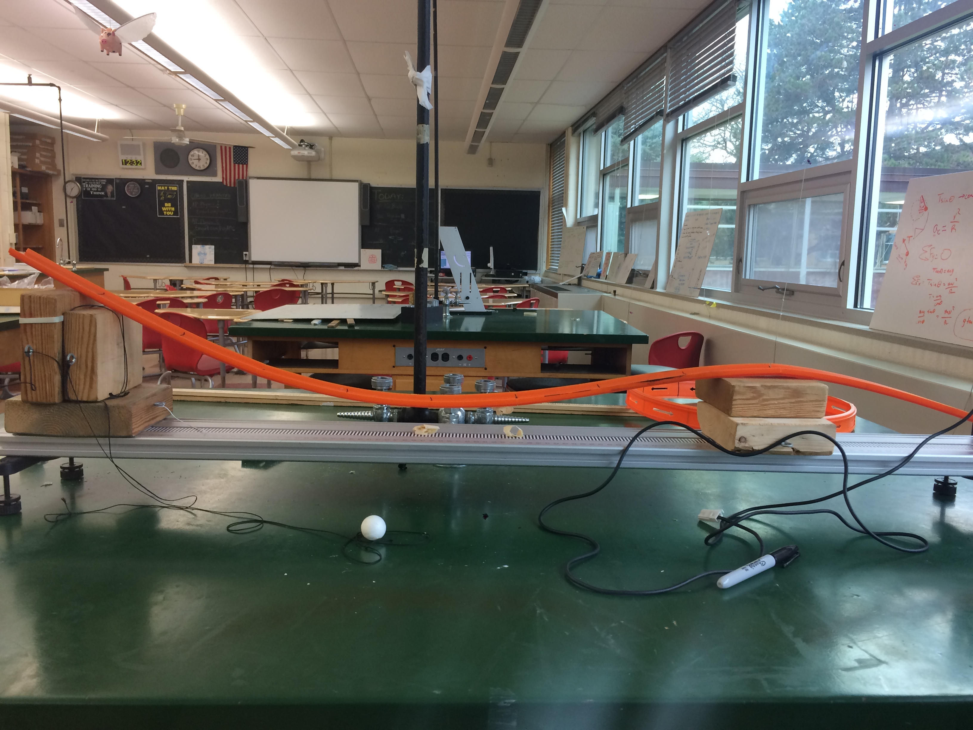
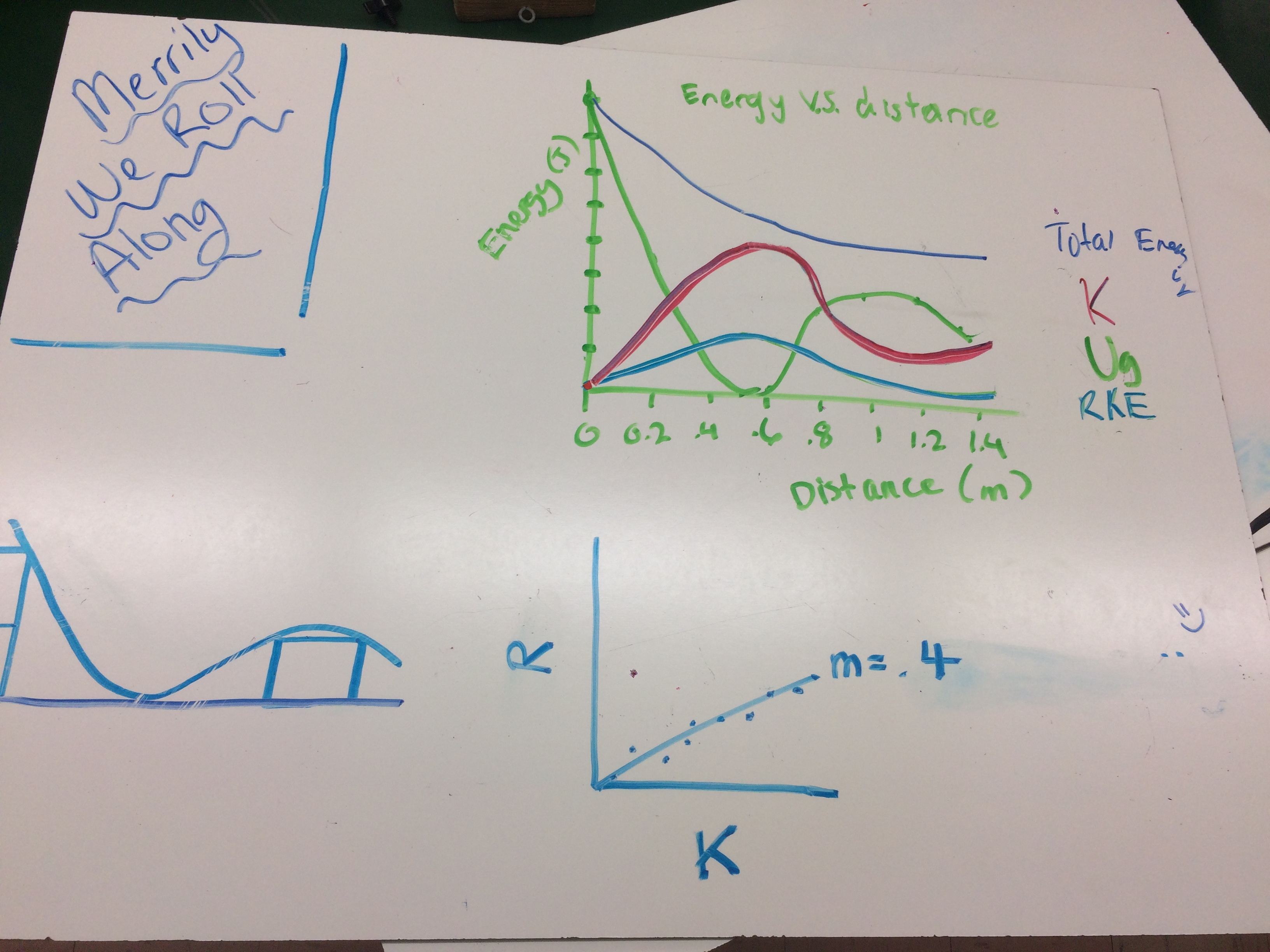
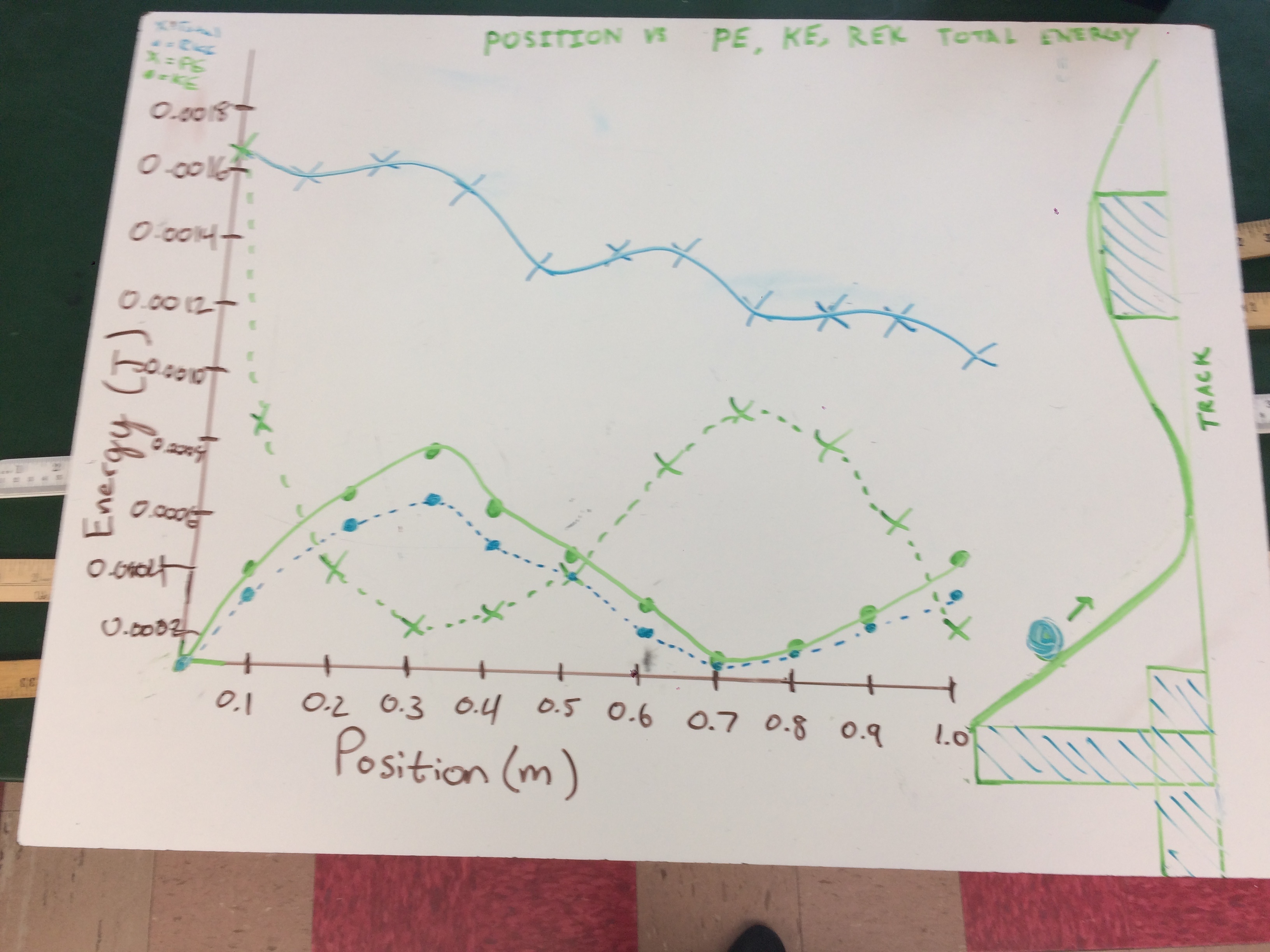
Do you notice anything? The largest drop off in TME corresponds to the moment where the ball is at the bottom of the hill. This serves as a great review of work and circular motion. Frictional force, as we know, is dependant on normal force. The normal force of the track changes and corresponds with its shape. We can actually predict the drop-offs in TME based on shape and even determine the work done by friction.

  1. A group with “bad” data.

Their data wasn’t actually bad, they obviously had forgotten something when they set up their formulas in the spreadsheet. But was there a way to find this without redoing the whole data spread? Absolutely. After creating a large circle to share whiteboards, we honed in on the group where the TME curve was mirroring the potential energy curve. The rest of the data seemed good…there was an obvious trade-off of PE and KE…although the curves weren’t as high as they should have been. So what was the problem? I selected a student to draw in where the energy curve should be, based on the shape of their track and everyone else’s data. She drew in the curve. Next, I asked students to note where this curve was and where the PE curve began. It was at 0.3 J with PE starting at 0.6 J Then I asked them to note where the KE curves were at… they were at 0.03 J. Notice anything??? They were off by a factor a 10! Where could a factor of 10 be? Did they forget a 9.8? Did they convert grams to kilograms properly? cm to m? Upon examination of their equations, they found the missing 10 and…TA-DA! Fantastic results.

I think it’s really important to note the value of both exercises. The lab itself was relatively simplistic, but it lent itself to fairly complex conversations.  I think this is especially true for the group with the “bad” results. How often do our students present with this and either (1) Default to “well my data must be bad” or (2) Start from scratch, rather than locating the mistake? In this way, students were able to critically analyze, strategize and problem-solve. It turned out to be a really easy fix.

Oh and the slope of the translational vs rotational KE? Yea that came out to 2/5….exactly. That’s super exciting!

Teaching Methods

Radical Renovations: The iOLab

I visited my alma mater today. The entirety of Green Street on campus is closed to traffic due to all of the construction. Buildings have gone down and come up and I half expected time to still be frozen in the year 1967 in the physics building.

When I walked in I found quite the opposite. Not only newly renovated rooms, but there is actually a women’s bathroom on the fourth floor. (This was always a running joke)

The reason I spent 6 hours in my car today, however, was to visit the Physics 101 class. iolab_remotes_red
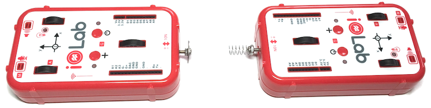
My former adviser, Mats Selen, has been working on a new project: the iOLab. The concept is simple, it’s a multisensor system in a box. And it can do everything your $10,000 of Vernier equipment can do… for a little over $100. It connects wirelessly to your computer and runs with free, opensource software that does all of the analysis our expensive programs run.

On the other side of the coin, however, is a radical change in how the introductory level classes are being taught. When students walked into the lab, they had done a pre-lab experiment earlier…..at home…..with their iOLabs. Quite simply, they made a stack of books, put another book on top by its edge and then looked to see how the force changed with the iOLab as it was placed at different distances from the book stack. Data were submitted ahead of time for credit. Students discussed the results at the beginning of the lab and then were given their task. It’s the classic peg-board demo, however, students had to find a way to relate the force to the placement of the probe if the pivot was located in the top corner.

This was the sum total of the direction given to students.

Within about 20 minutes all students were taking measurements. Some were looking only horizontally, others were looking both horizontally and vertically. Questions arose about the approach: if we change the angle at which we hold the probe the force will change. Are we supposed to do this with a horiztontal force too? I think that’s impossible.

They were told it’d be great if they came up with a mathematical relationship, but they’re just looking for the trends.

Within an hour students were plotting their data, recognizing it was an inverse relationship and running the curve.

One group really wanted to get the formula.

Another group recognized the torques should be equal and started calculating all of the torques. Percent uncertainty was one of the objectives focused on, so I wanted to see how well they were grasping that concept. I looked at the torques and noticed the values were .14, .14, .14, .15, .16. So I asked them how they were going to decide that those were constant and not increasing. They responded that they would have to determine their percent uncertainty and compare what was acceptable to those values.

Now, clearly there are major differences between high school junior and seniors and pre-med juniors and seniors, but at the same time, it was still remarkable how they were approaching the lab, developing their experiment and writing up their labs. It is something that very much excites me about the potential use in the high school classroom (and online classrooms, and college classrooms etc)

I also asked students about their previous physics experiences. About half reported they had taken physics in high school, ranging from regular level to AP Physics 1. ALL students reported that they felt they had a FAR BETTER grasp of physics now in this course, compared to their high school course. Several students who said this felt the need to insist they still had a great high school teacher 🙂

The message, however, is clear: we need to give our students the opportunity to design and evaluate their experiments.

Also, the iOLab is a very exciting new piece of equipment. Morten Lundsgaard, currently the Coordinator of Physics Teacher Development
Instructor, is hoping to run workshops and/or a camp for high school teachers. If you are interested you should contact him!

Concept Modeling · Teaching Methods

Slicing a Cylinder for Moment of Inertia Integration

Guys….we’re in the throws of rotation. And at least one of my poor students has calculus immediately preceding AP Physics C. I feel so bad for her. The day we started she had made up a calc quiz, came to day 1 of rotational inertia, then went to calculus. Oh did I feel her pain.

Arguably the most difficult part of deriving rotational inertia is the visualization of how to go about the integration. I mean, let’s be honest, once we find how to express dm the integration is always an easy one.

Part of the problem is getting students to understand what it means to say things like dm, dV, dA, etc. They understand the definition linguistically, but it’s really hard to think of it practically. Tell them that dr^2 is zero and their minds are blown and bothered.

Day 1 of cylinders did not go well. Arguably, in part, because we were short on time. But also because the what why how was overwhelming.

I remembered a demo someone had shown where they 3D printed their objects to roll down the incline. They had actually made nesting cylinders, which then served as a great way to discuss integration.

I’m trying to think of a way to visualize each of the d-steps of the cylinder integration for my students with materials I have on hand. As I’m digging through the closet I notice the slinky coil. It’s nearly perfect!!!

Ideally, I wish I had one with nice thick coils so we could take about the cylinder with R1 and R2, but this will suffice for the most challenging part.

So imagine you have a cylinder of length L, and inner radius R1 and outer radius R2 and would like to determine the moment of inertia about its center…

IMG-2037 (1)

First, as always let’s define rho, but we have to find dm in terms of r. So how do we do that?

Well, let’s take some horizontal slices, where each slice is dm… now we can see that dm = rho*dV…but wait… what is dV?

Well, if we make those slices infinitely small…is there really a volume left?

IMG-2040

Ah! so dV is really dA, and we are looking at it across the length of the slinky, so dm = dA*L!

Conveniently, I know that A=pi*r^2, so dA = 2*pi*r dr

And the rest is substitution!